Circuit Notes: A Simple Pulse Generator
Update (Oct 11, 2015): I added my schematic file and netlist in case you want to play around with this circuit on your own local LTSpice install. It’s free, so you might as well!
I’ve been slowly working my way through Horowitz and Hill’s Art of Electronics, 3rd Edition as a way to refresh and sharpen my analog electronics knowledge. Most of my professional life is about stringing together complex ICs, and not enough about the building blocks of electronic circuits. I figured that I’d take the more instructive examples from AoE and publish my workthrough of them here. Expect some dry prose, some scrawled notes on engineering paper, and maybe a simulation or two as I see fit. (I’m currently using LTSpice for Mac, but I’m not wholly enamored of it. Any suggestions?!)
A Simple Pulse Generator
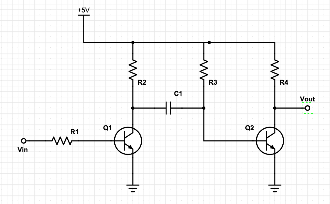
Figure 1: A Pulse Generator
The purpose of this circuit is to provide a quick pulse at output Vout when stimulated by a rising edge at Vin.
###Notes on DC Conditions
- Q1 is off, meaning VQ1-C is effectively 5V.
- Q2, however, is on. That places VQ2-B at approximately 0.7 V, and VQ2-C/VOut at ground.
- Note that the on/off states of Q1 and Q2 combine to produce a voltage of about 4.3 V across C1.
###AC Analysis Suppose we stimulate Vin with a rising edge of 5V. This will turn on Q1, the speed of which is limited only by that transistor’s turn-on time. It’s important to pick R1 such that you can guarantee Q1 entering a saturation condition; we want this transistor on when Vin drives high!
This quick turnon of Q1 will drive the collector voltage, VQ1-C, to ground. Note the DC state of C1 - it’s still retaining the ~4.3 V charge it acquired while the circuit was at steady state. As a result, VQ2-B is now -4.3 V, shutting off Q2 and driving VOut to +5 V. You’ll note that, with VQ1-E being at ground, the combination of R3 and C1 are effectively forming an RC circuit, with the initial condition of VC1 = -4.3 V. \[V_{out}(t) = 5 - 9.3 * e^{\frac{-t}{\tau}} [V]\] \[V_{out}(t) = 0.7 = 5 - 9.3 * e^{\frac{-t}{\tau}} \Rightarrow \frac{(0.7 - 5)}{-9.3} = 0.462 = e^{\frac{-t}{\tau}}\] \[0.462 = e^{\frac{-t}{\tau}} \Rightarrow \frac{1}{0.462} = e^{\frac{t}{\tau}}\] \[ln\big(\frac{1}{0.462}\big) = \frac{t}{\tau} \Rightarrow ln\big(\frac{1}{0.462}\big) * \tau = t = 0.722 \tau\] \[0.722 \tau \approx R3C1\]
Basically, this shows us that we can set the “on” time of the pulse using R3 and C1 similar to choosing values for an RC circuit. Cool!
Notes on AC Performance
The first thing this circuit assumes is that Vin is going to drive high and stay high. What happens if the input pulse is shorter than R3 * C1?
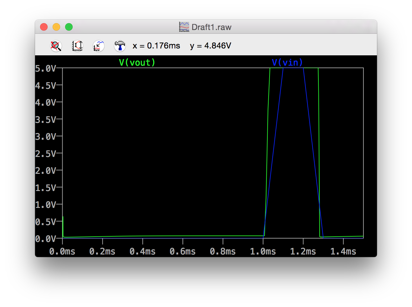
Figure 2: Pulse Generator Output where Vin is high shorter than Tau
The simulation above shows an LTSpice representation of what happens to this circuit when the input pulse is less than the time constant. The output pulse will get shortened in turn - as soon as Q1 is back to its normal off state, C1’s charge will be polarized in the opposite direction of DC steady state. This will just assist the 5V rail in keeping Q2 on, and shortening the output pulse. What if we want a pulse at Vout that is always R3 * C1 in length? We’ll need to decouple the output from the input. This is easily achieved with another transistor that monitors the output of the circuit.
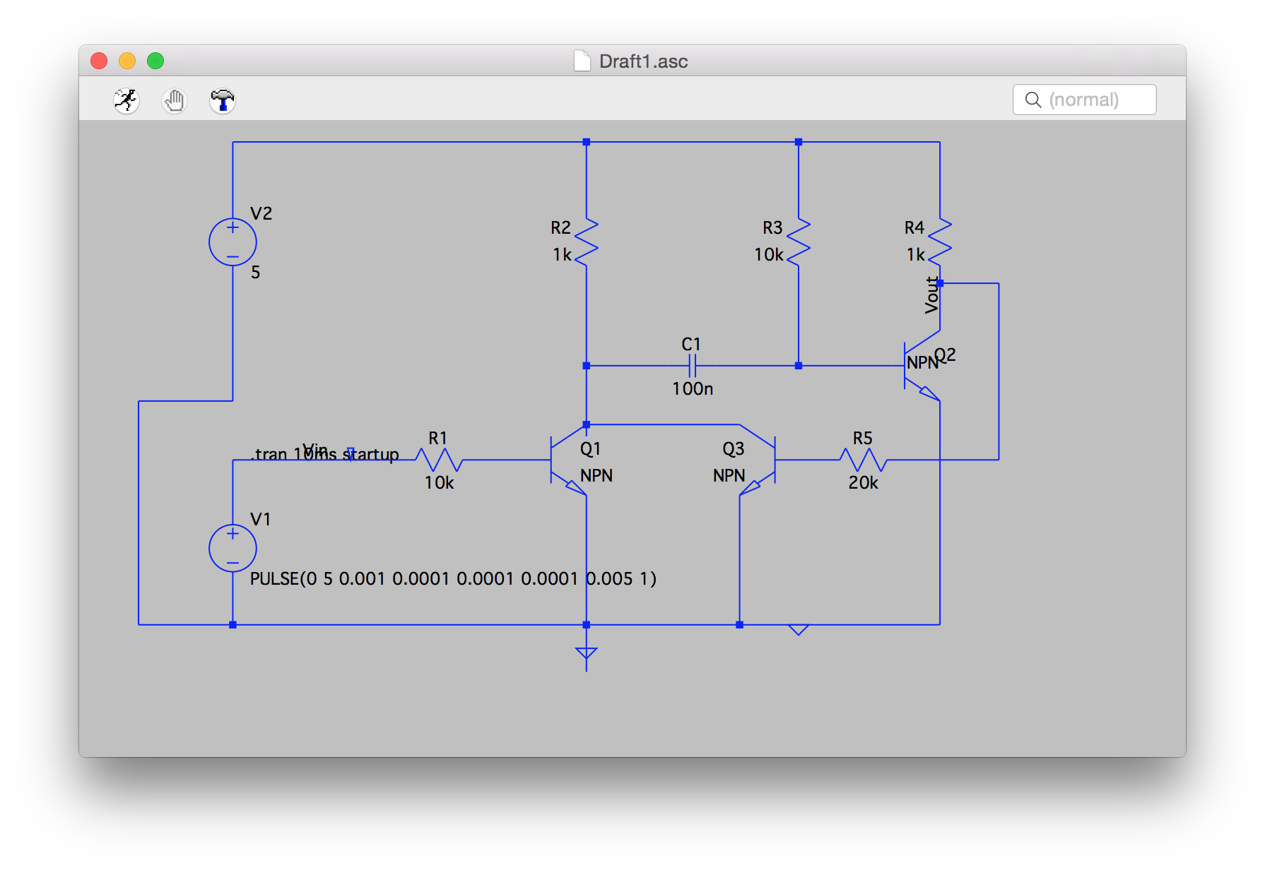
Figure 3: A Pulse Generator w/ Guaranteed Pulse Width
Q3 serves the purpose of holding VQ1-C to ground once a rising edge is detected at the base of Q1. As long as the input pulse is as least as long as Q1’s turn-on time, the circuit will work properly. This is due to the fact that, once Q1 has successfully driven VQ1-C to ground, Q3 will also be turned on, providing another path for the R3/C1 circuit to be held at ground. Figure four shows this improvement in the output pulse width.
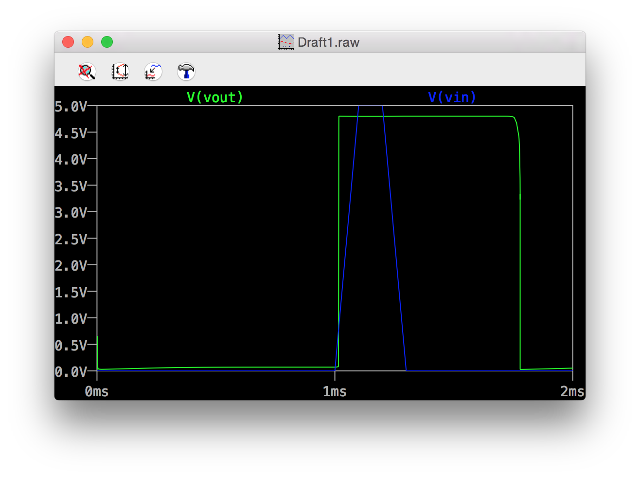
Figure 4: Pulse Generator Output with Guaranteed Output Width
The addition of Q3 made circuit performance a little bit easier to predict by allowing us to modify pulse width by changing the values of C1 and R3. It wasn’t a silver bullet, however. Figure four shows that the falling edge of the pulse isn’t nearly as sharp as the rising edge. There’s a distinctly rounded corner at the beginning of the falling edge, which is a result of the leisurely voltage transition of the R3/C1 through Q3’s turn-on voltage. There’s not a lot we can do to this circuit to speed up this transistion without affecting the pulse width. Instead, we’ll need to change the output drive strength with another small addition.
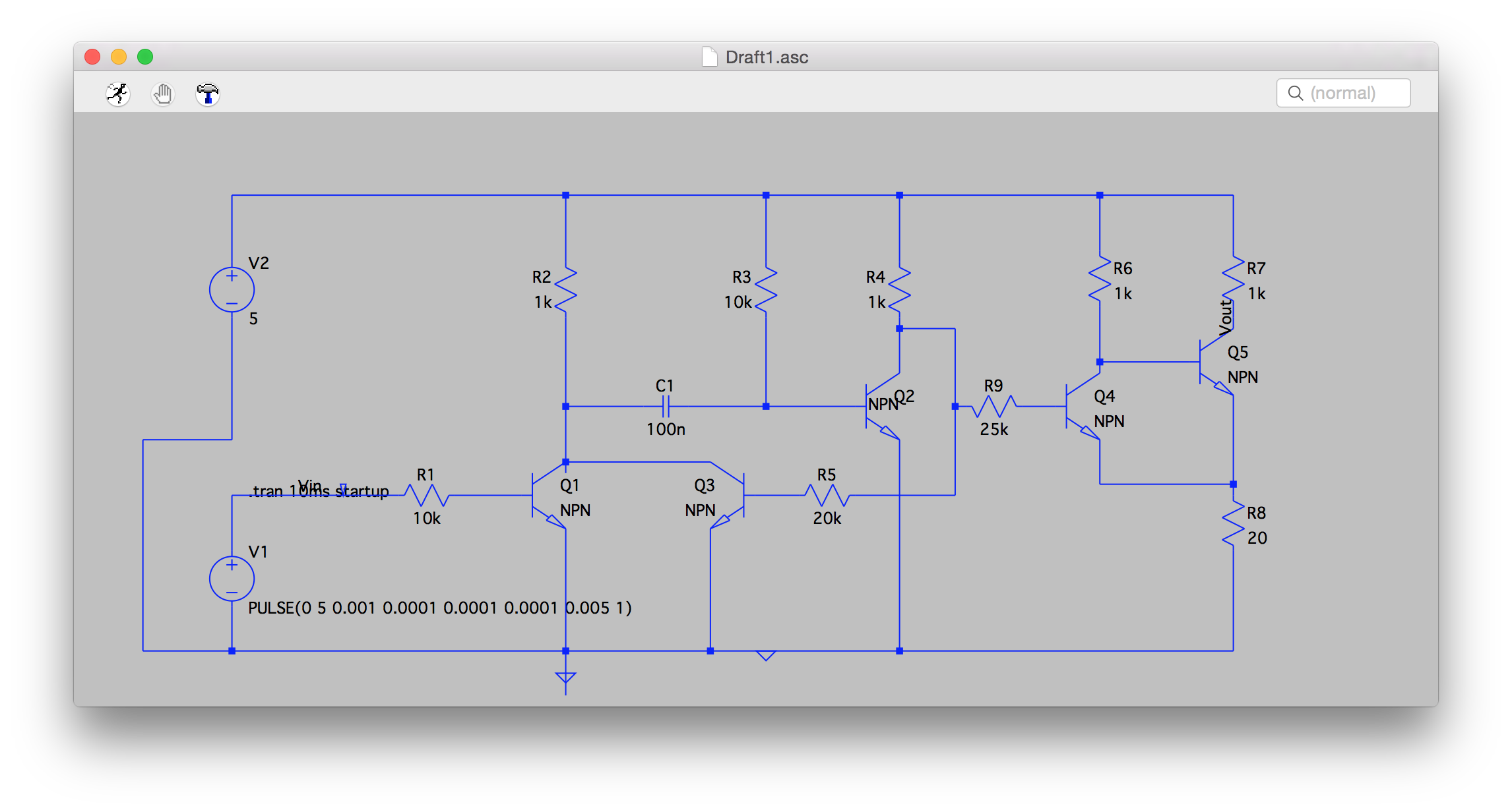
Figure 5: Pulse Generator Output with Schmitt Trigger Output
This output stage is a Schmitt trigger, which is a handy little circuit for cleaning up slow or noisy edge transitions. Going to the simulation shows that it’s done the trick for us:
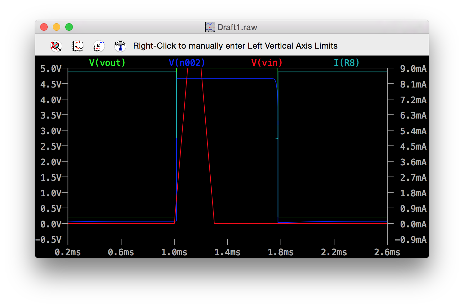
Figure 5: Pulse Generator Output with Schmitt Trigger Output
This is all well and good, but you’d never use this circuit in a real application. Why? Power! Check out the current through R8 alone. That single circuit leg is peaking at around 9mA while Q5 is on. Most modern ICs draw far less current than 9mA. Many modern DRAM devices - components with billions of transistors - manage to consume less than 100 microamps in self refresh states. That being said, it’s a fun little circuit, and reasonably easy to build for instructive purposes.
Acknowledgements
I pulled this circuit and its improvements out of Horowitz and Hill’s excellent Art of Electronics, 3rd Edition. You can check it out on page 77.